Basic Stats

In this section, we’ll explore frequentist statistics, more commonly known as just ‘statistics’ or hypothesis testing. Hypothesis testing let’s uncover if different treatments cause the same outcome. A treatment pre-defined by one or more dimensions. You maybe familiar with treatment in the context of medical studies. One group of patients might receive an experimental medication while another gets a sugar pill. The study would try to measure if the new drugs have the same effect as the placebo. The analyst will run a hypothesis test (more on these soon) to check if the two treatments are significantly different.

Traditional statistics definitely has it’s place in a modern data scientists toolkit. Not only as the precursor to machine learning but also as a powerful tool in-and-of itself.

Before going too far, we have to address the fight between Bayesian and Frequentist statisticians. If you aren’t familiar, these two camps have been engaged in a bitter debate that frankly doesn’t really serve anyone. Both approaches have a large amount of value in the correct context. We’ll talk about both.

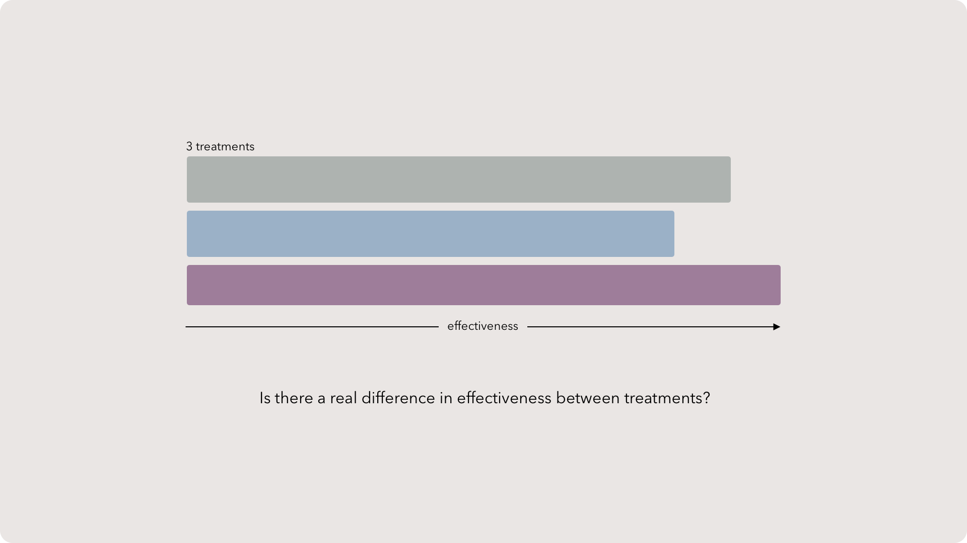
Measuring the effect of different treatments may seem like a simple task. Surely, we can tell if treatments have different centers — either mean or median — then one must be better than another…

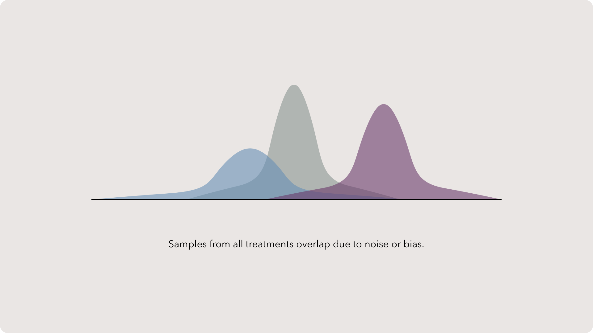
Unfortunately, this is isn’t the case for a few reasons. Each treatment will be composed of several samples that all have noise and bias making them estimates of the real value. Hypothesis testing takes into account the imperfections in our data to try and determine what the probability of seeing a result is. We’ll use the distributions from each treatment to test our hypotheses — more on testing in a bit, first we need to understand distributions.

Distributions are the represented by a value on the x-axis with the frequency on the y-axis. The more a value occurs in the data set, the higher the peak around that point in a distribution.

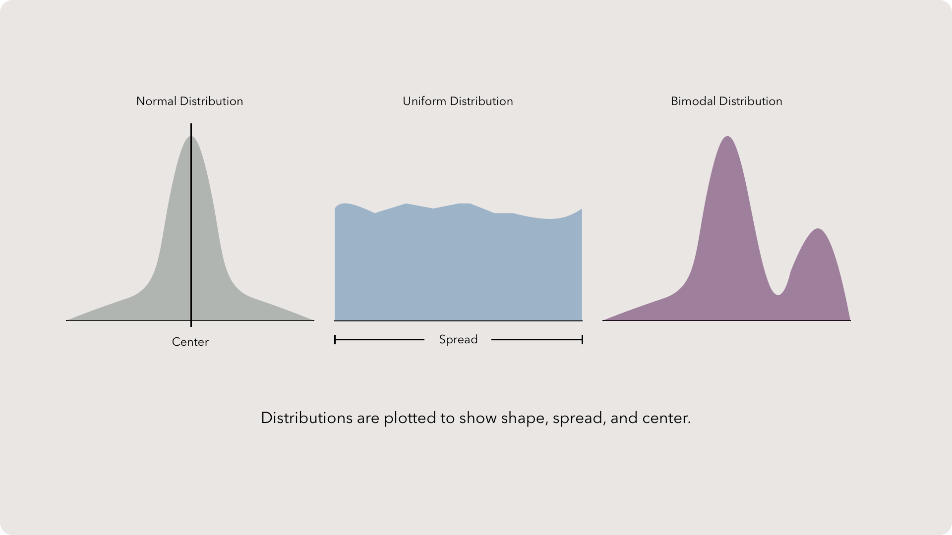
Keeping in line with this course, this isn’t a comprehensive discussion of distributions. I want you to get a feel for numeric distributions but note that categorical distributions also exist.

We describe distributions with three key attributes: the center, the spread and the shape.

The center is your typical measure of central tendency. This is either the mean, median or mode. As we’ll see in a second, median is a robust measure but most folks use mean simply since its more commonplace. In case your brain is foggy, the median is the middle value of when you line up all the data in order.

Spread represent the range of values. Think about the distance between the minimum value to the maximum and that is how far the data spreads out.

Finally, shape. Your data will in all sorts of shapes when you plot the distribution. However, it is extremely common for the data to form a normal distribution, or bell curve. This distribution has a large bulge in the center than descends rapidly and spreads out in tails. The law of large numbers describes the natural phenomenon where the more data is collected from a population, the closer the sample space will look like a normal distribution.

You might also encounter uniform and bimodal distributions as well. Uniform distributions occur when the data has roughly the same frequency. Think of a plateau, where every value is equally likely to occur. Bimodal distributions are like normal distributions, but have two peaks. Yes, you might have multi-modal distributions but that likely indicates your are not creating proper treatment groups.

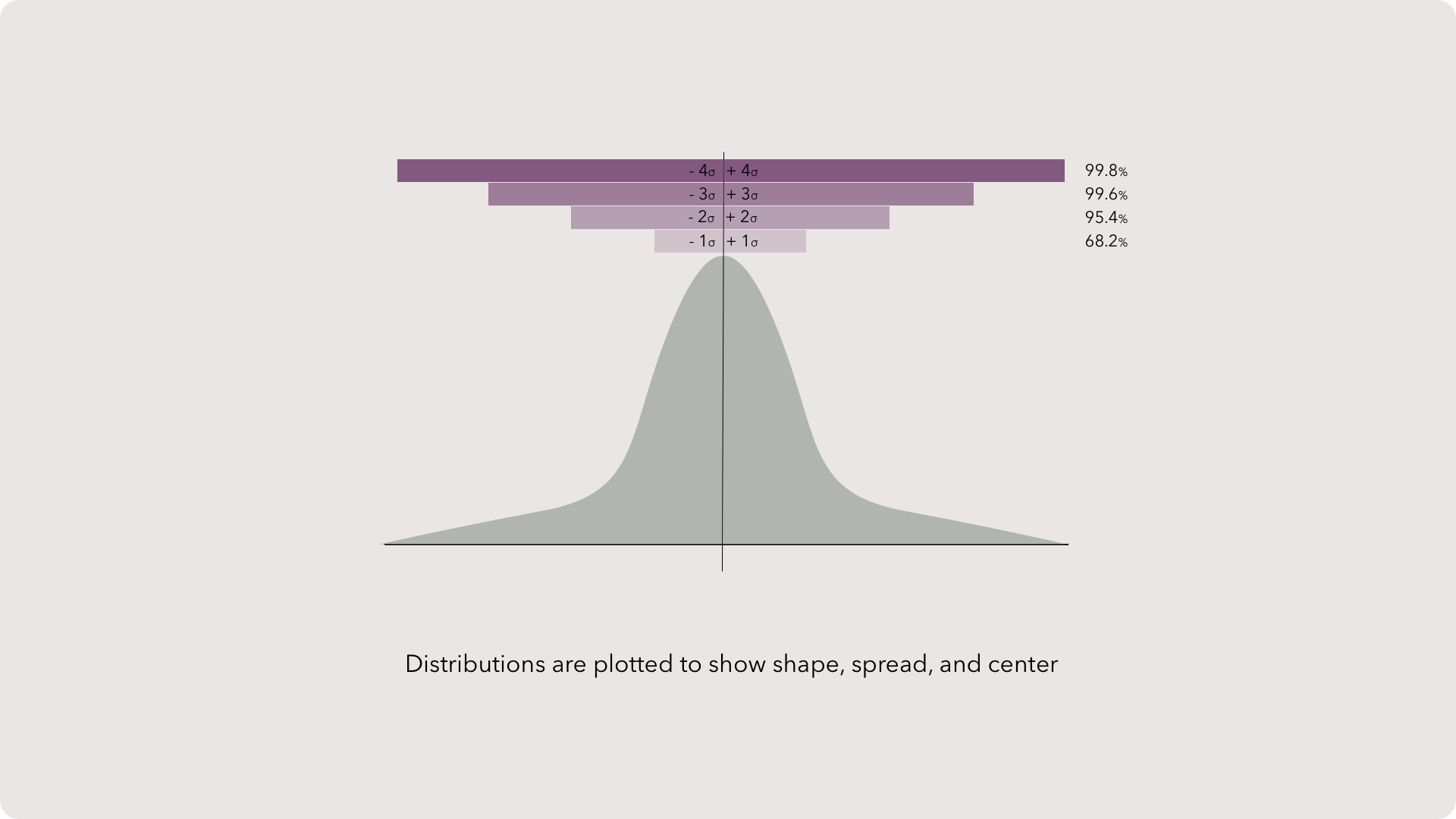
Standard deviations are the average distance between a given data point and the average value of the metric. Typically, you want low standard deviations since that indicates that the data is tightly packed together. Tightly packed data is great for controlling processes or using a variable as control knob in experiments.

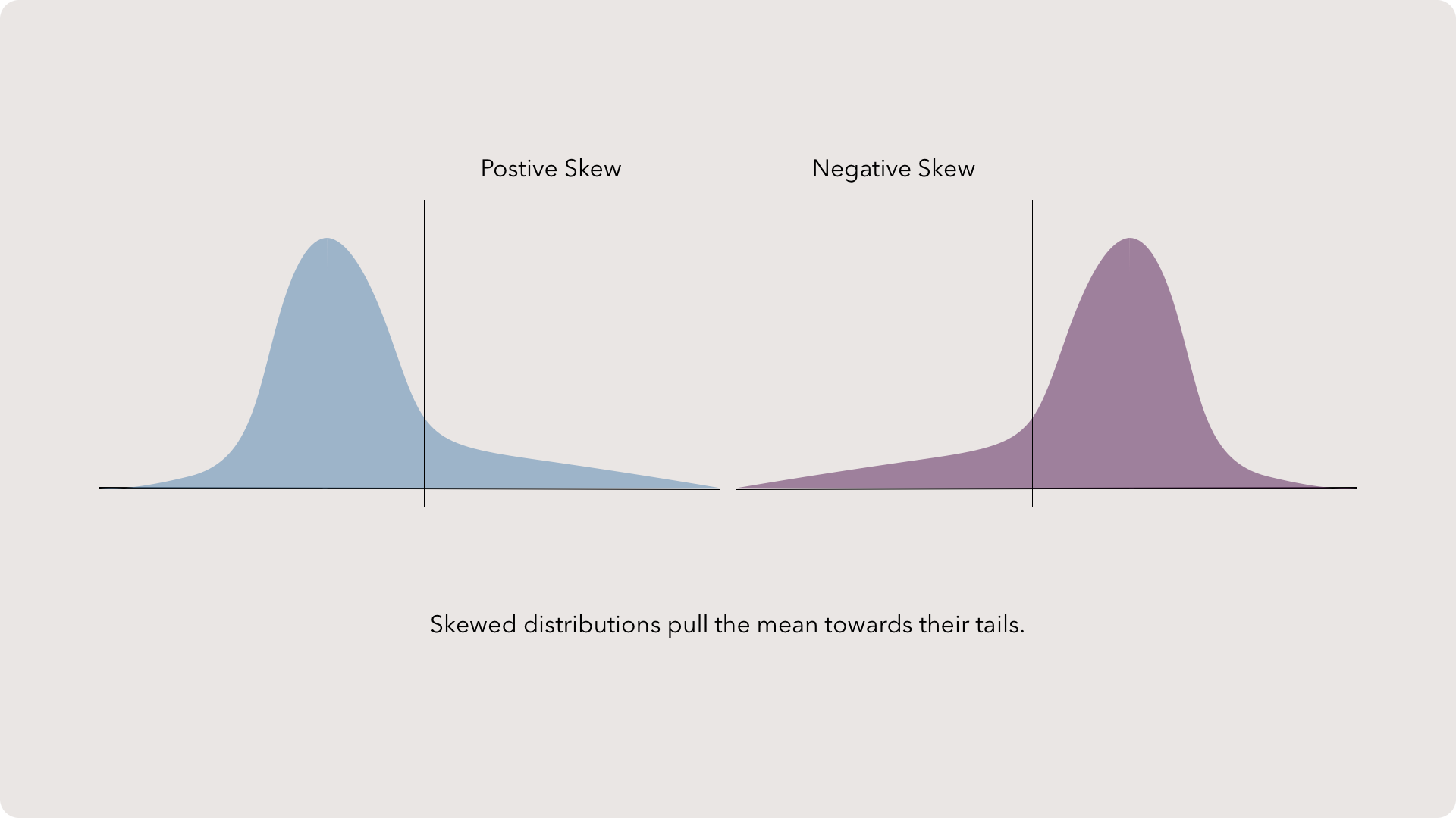
Data shapes often have a tilt or bias that are called kurtosis, or more commonly, skew. You can recognize skew in a histogram by a long tail that moves away from the body of the data. There are two types of skew, positive skew with the tail on the left and negative skew with the tail on the right. Skew pulls the mean away from the median, making the mean values more susceptible to outliers. This means that one-sided, long-tailed (aka skewed) distributions will pull the mean towards the tail. Pulling the mean away breaks many statistical tests rest on the assumption that the mean is the center of the distribution.

To make a firm statement about what the data is telling us, statisticians produce a formal statement called a hypothesis, which is an idea based on existing experience that can be tested.

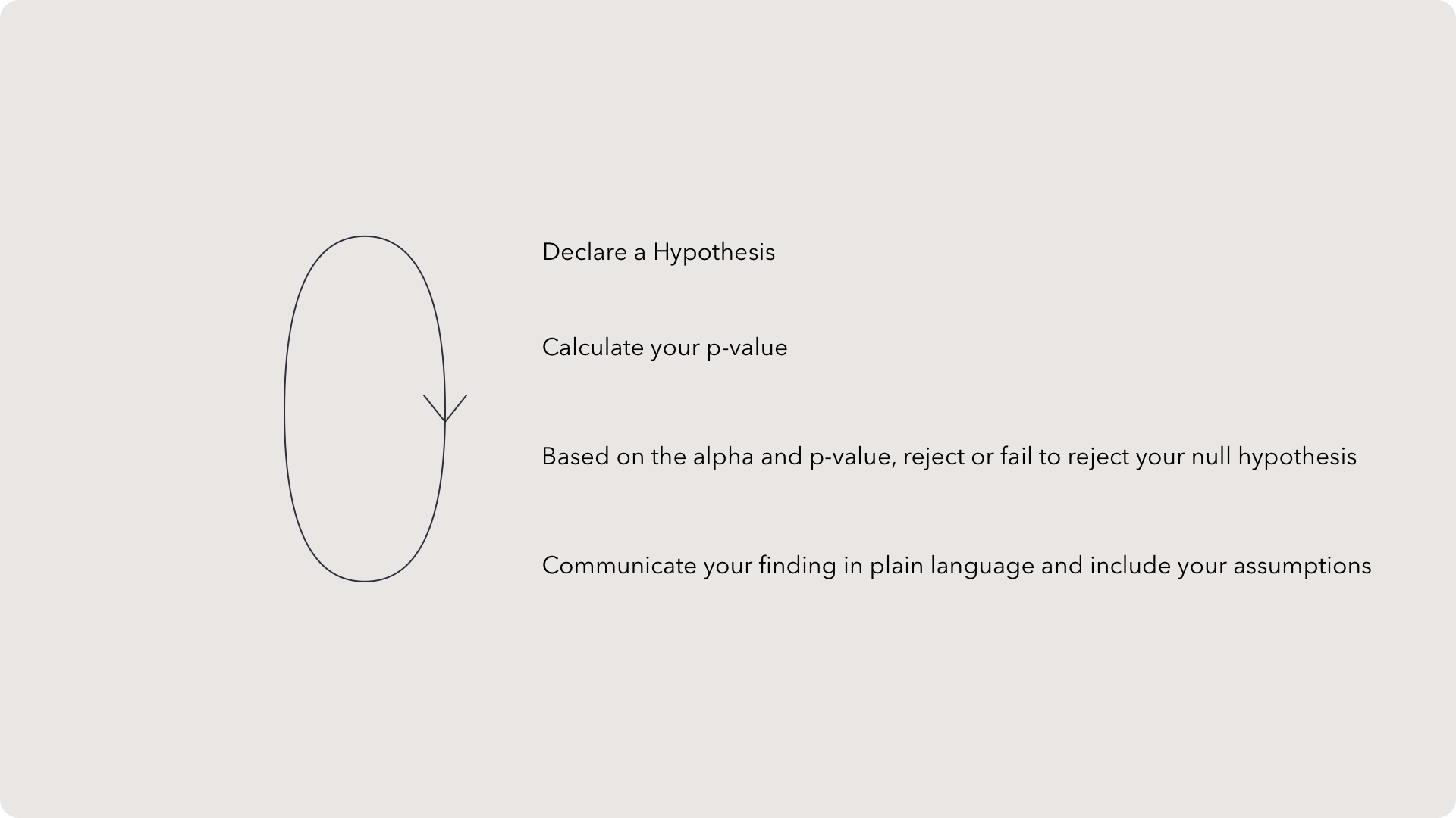
Hypothesis testing is broken down into four key parts. First, we need to declare a hypothesis and its alternative — more on this soon. Then we use our data to calculate a p-value. The calculation doesn’t really matter for this short course as your software will have this built-in. We compare our p-value to the alpha (again, more soon), and decide if we can reject our null hypothesis.

Let’s slow down that interpretation. In statistics, we can’t “prove” anything. Chance and bias always play a role in how our data can be interpreted. Instead, we can make statements about the likelihood of our statement being supported by our observations opposed to just seeing our results by chance. Imagine you win the lottery, it would be inaccurate to state that winning is easy or common. You just got very lucky. The rejection of a hypothesis uses safeguards so a researcher must state how likely the results of a treatment would be similar result would be due to luck alone.

Finally, we communicate our findings back in a way that any audience could understand. Don’t skip this step. Please don’t. Your job is to help people learn new things about the universe, not hoard knowledge behind archaic formulations.

A hypothesis cannot be “proven” in the traditional sense. Instead, we would make a null and one or more alternative hypotheses, denoted as Ha formally. The null hypothesis, symbolically represented as Ho, simply states that a difference was not observed between each treatment. Likewise, the alternative hypotheses claim that the treatments differ significantly, more on that below. The classic example of null and alternative hypotheses is from pharmaceutical research. Suppose you are studying a drug’s effectiveness. You might have a placebo group as a control, which essentially is a sugar pill, and a new drug Cureol. Your null hypothesis would be there is no difference in disease recovery between the control and experiment treatments. The alternative hypothesis would be the flip of that: there is a difference in disease recovery between the control and experiment treatments. You would test the data based on these hypotheses and determine if the null hypothesis can be rejected.

We use the phrase “fail to reject”. Because we cannot absolutely prove a hypothesis, we must either support or not support it based on whether we can negate it. If we reject the null hypothesis then logically we must support the alternative hypothesis. If the null hypothesis cannot be rejected then there is not enough evidence to support the alternative hypothesis.

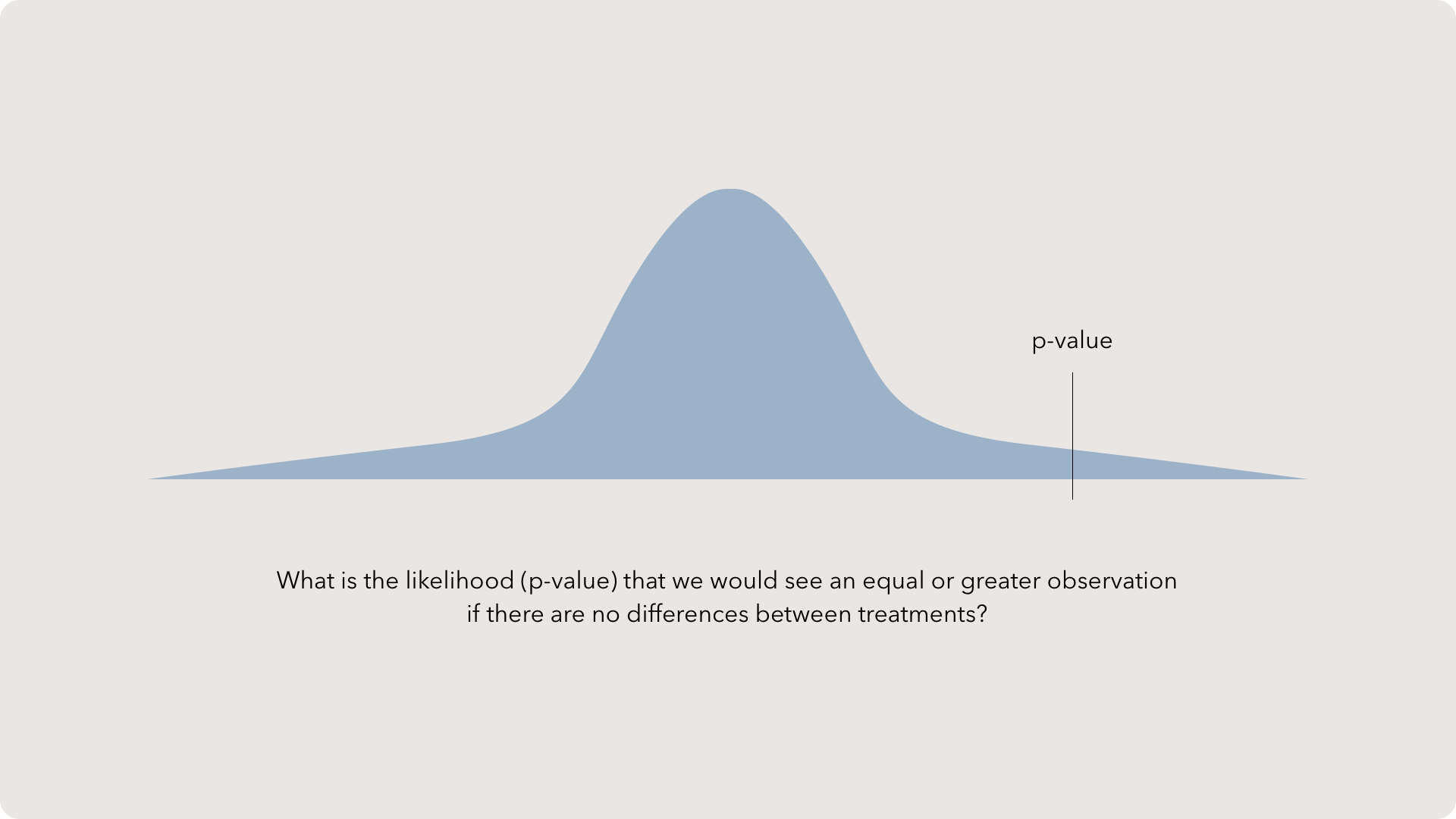
We don't specify any magnitude of change in the hypothesis itself, but instead we look at the significance level , known as the alpha a, which represents the amount of risk the researcher is willing to take in failing to reject the null hypothesis. Traditionally, researchers use an alpha of 0.05 or 5%, so we’ll use this too. An alpha of 0.05 indicates a 5% chance of rejecting the null hypothesis when one should have failed to reject. When we test our data, we'll compare the result to this alpha value, and that will determine which hypothesis we must accept or reject.

Note: This alpha value is entirely arbitrary and a valid criticism of Frequentist statistics. Some scholarly journals are even disallowing statistical interpretation based on significance.

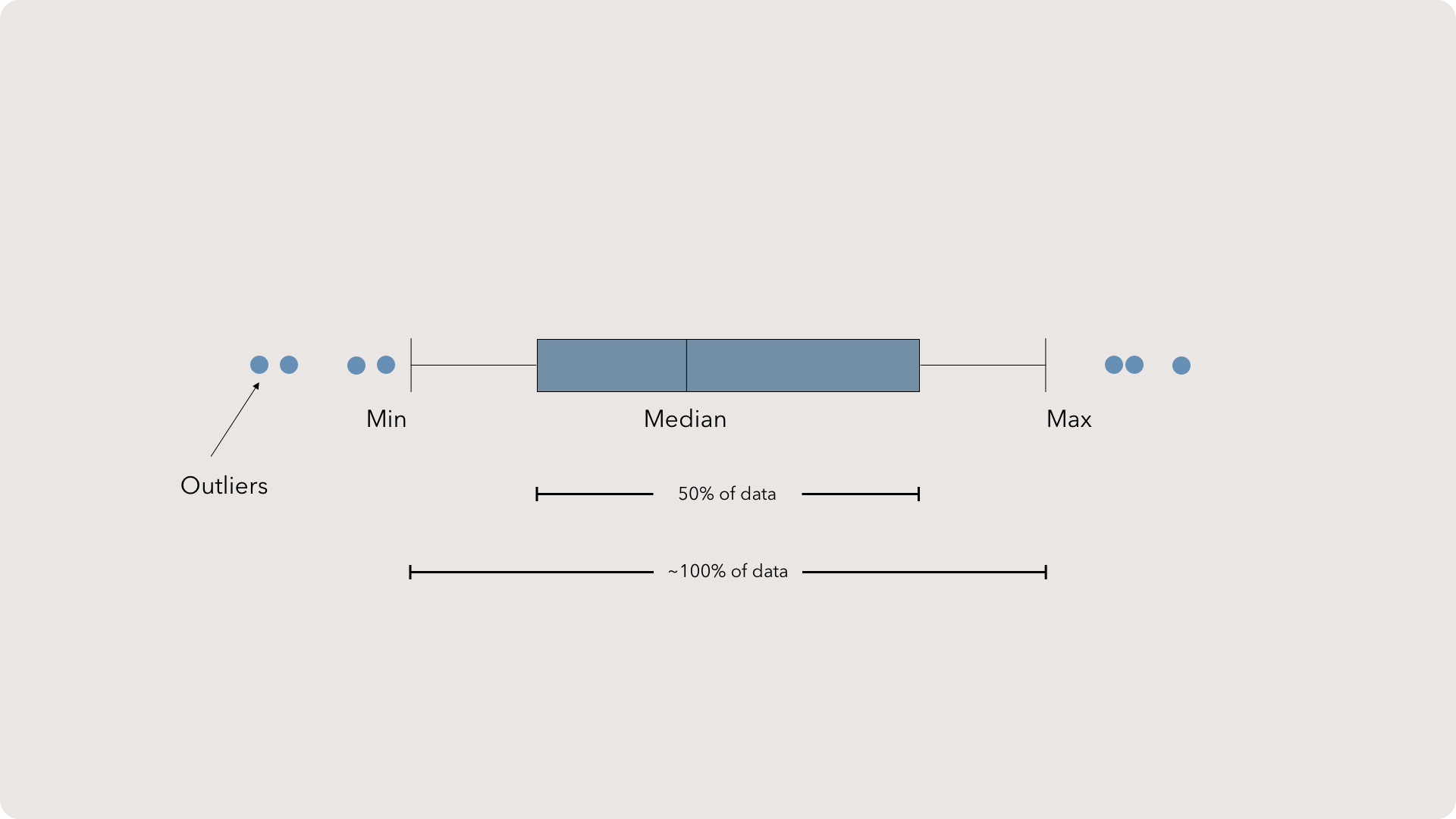
Confidence intervals (CIs) are an estimated range of values around the metric’s center, typically the mean. A CI indicates the range of values in which the “true” value could occur. Think of the CI as a safe bet. The value that is most representative of the population at large should be in the CI.

Commonly, scientists use a 95% confidence interval range or plus-and-minus two standard deviations. This protects the CI from most outliers while providing the maximum amount of range for analysis.

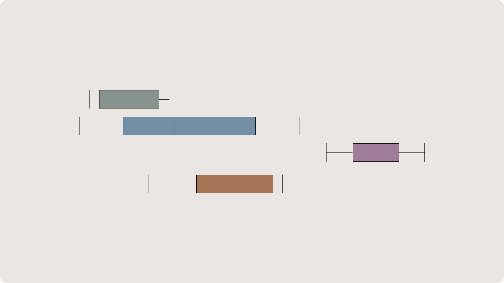
P-values receive a lot of criticism, for now obvious reasons. While traditional statistical tests have a lot of value, there is a solid argument for the use of confidence intervals instead of p-values.

Confidence Intervals can be used to replace hypothesis testing with p-values. This has the advantage of being simpler to understand. If the confidence intervals don’t overlap at all then you have evidence suggesting that the two groups behaved differently. Likewise, if the intervals overlap over the center, then there is evidence supporting no difference between groups.